11 Detection of archaic ancestry segments using admixfrog
11.1 Archaic ancestry
Neandertals and Denisovans lived in Europe and Asia for hundreds of thousands of years before their disappearance around 40 thousand years ago (kya) (Higham et al. 2014). In the last few thousand years of their documented existence, they met and interbred with modern humans who arrived from Africa, and as a result, 2-3% of the ancestry of present-day non-Africans derives from Neandertals and between 0.2 to 4% from Denisovans ((Green et al. 2010),(Reich et al. 2010),(Meyer et al. 2012),(Prüfer et al. 2017), (Hajdinjak et al. 2021)).
Genome-wide average archaic ancestry can be detected using F-statistics or D-statistics ((Peter 2016)). However, for more detailed investigation of the archaic ancestry in the modern human genomes, segment calling is preferred.
11.1.0.1 What can we learn from the segments?
Number and duration of the introgression event(s)
Generations past since the introgression event
If the archaic segments in different individuals result from the same introgression event or not (Iasi et al. 2024)
Selection, functional consequences..
Hidden Markov Models (HMMs) are used for calling the archaic segments, and there are various methods including hmmix which is reference free method that currently do not work on low coverage data (Skov et al. 2018), and other HMMs which can detect segments using genotype calls (again, not suitable for low coverage data) (Prüfer et al. 2021). In this chapter, we will focus on admixfrog (Peter 2020), as it can call segments in low and contaminated data.
11.2 Calling archaic segments with admixfrog
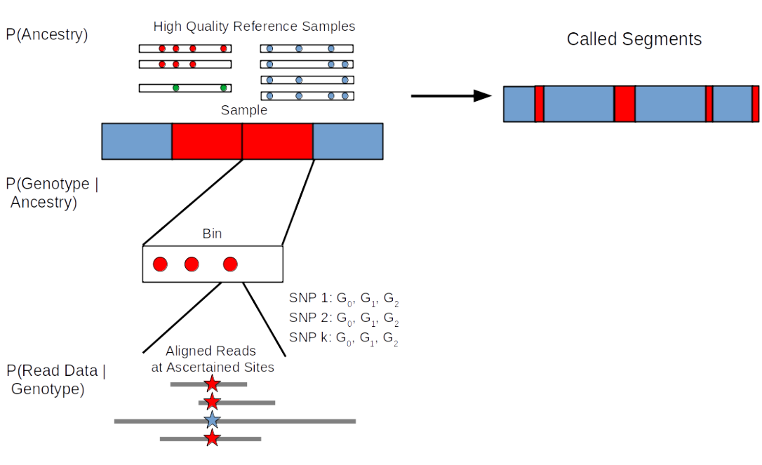
Admixfrog can call segments of archaic ancestry from unphased nuclear genomes with coverage as low as 0.2x, both from shotgun and capture data. It is well tested on not only detecting Neandertal/Denisovan ancestry in modern human genomes, but also for detecting Denisovan ancestry in Neandertal genomes. Admixfrog is a HMM with hidden states being all possible pairwise combinations of ancestry between user defined source populations. The method does not rely on simulations and model assumptions much, and uses the data to estimate parameters with a flexible Bayes model. It requires two main input files:
Target genome that belongs to the individual one wants to detect archaic ancestry in. This file can be created from a bam file using the command admixfrog-bam. Alternatively, if contamination and error should not be estimated, it is possible to use genotypes provided in eigenstrat-format. It contains observed number of alternative and reference reads, and is stratified by read length, library ID, and presence/absence of deamination on the read.
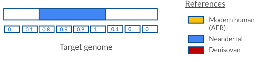
Reference file that includes the high coverage genomes of the “sources” admixfrog uses to model the ancestries in the target genome. This file can be created from vcf files using the command admixfrog-ref. Reference file is very important and should be generated carefully. If capture data is being used for the “target”, reference file should also be ascertained with the same capture sites. The assumption of admixfrog is that the source genomes are unadmixed. It contains the counts of alternative and reference alleles for all reference populations, and specifies the genetic map that is used.
When these two input files are provided and various parameters (such as bin size, states, recombination map, run penalty, error rate..) are specified, admixfrog splits the target genome into bins of a given size and estimates the probability of (homozygous or heterozygous) reference ancestry (combination) for each bin. It does that from the genotypes in the bin by estimating the probability of observing the target genotypes given a reference population. If genotypes are not available, admixfrog can estimate the genotype likelihood from the read date, while taking contamination into account. For this, it uses a genotype likelihood model :
\(P(O_r|G, c_r, n_r, e_r, p^c) ~ Binom(O_r; n_r, p)\)
where \(p = (1-e_r)p'+e_r(1-p')\) and \(p'=c_rp_c + (1-c_r)G\).
The contamination is estimated from the observed allele on the reads (\(O_r\)). The reads are clustered into read groups (\(r\) with \(n_r\) reads in the read group) which stem from a certain sequence library, with a given length and presence or absence of contamination. From this the proportion of contamination (\(c_r\)) and error (\(e_r\)) is estimated. The basic idea here is that if there is no contamination \(,p\) the probability of seeing a derived allele, should be the same across all read groups for a certain SNP. If there is, however, contamination and error it will lead to variation between read groups from, which the error and contamination parameter can be estimated.
11.2.0.1 Installing admixfrog
Admixfrog requires python version 3.8 or higher, along with several packages. Dependencies can be installed with pip install cython scipy --upgrade and admixfrog can be installed from github with pip install git+https://github.com/benjaminpeter/admixfrog.
More information can be found in the github page, installation explained in: https://github.com/BenjaminPeter/admixfrog/tree/master.
11.2.0.2 Preparing input files
- Target file
If you have called trustworthy genotypes for your target sample, you can use the VCF and create the input file:
admixfrog-bam --ref ref_example.xz --vcfgt {input.vcf} --target {sample_name}"
  --force-target-file
  --out {output.csv}
If bam file is being used, make sure the RG tag in the bam file is specifying the correct library the read came from (quite often not the case). Also if library is fully UDG treated it might me difficult to determine deaminations:
admixfrog-bam --bam ${target}.bam --ref ref_example.xz --out ${target}.in.xzThis file should looks something like this:
chrom  pos        lib                         tref  talt  tdeam  tother
1      847983     Lib.L.9150_0_nodeam         1     0     0      0
1      851309     Lib.L.9150_1_nodeam         1     0     0      0
1      853596     Lib.K.4356_1_nodeam         1     0     0      0
1      853962     Lib.K.4356_2_nodeam         1     0     0      0
1      858641     Lib.L.9150_0_deam           1     0     0      0
1      859871     Lib.L.9150_0_deam           1     0     0      0
1      867151     Lib.L.9150_0_nodeam         1     0     0      0
1      867404     Lib.L.9150_4_deam           1     0     0      0
1      872687     Lib.K.4356_0_nodeam         1     0     0      0
1      873541     Lib.K.4356_2_deam           1     0     0      0
...- Reference file
This file contains the population allele counts for the reference and alternative allele, for the reference populations the target genome is ‘painted’ with. This requires high quality genomes for accurate allele frequencies, especially if the number of individuals per reference is very small or even just a single individual. The closer the reference population is to the introgression population the better. If reference populations are themselves admixed (with one of the other reference populations), as many individuals as possible should be provided for a good inference. Usually only ancestry informative sites are used (sites where the are substantial frequency differences between reference populations or even differentially fixed sites). This also increases the speed of admixfrog.
For each site, the reference file contains the chromosome, physical position and at least one genetic map giving the genetic distance between sites. Using the command presented here the reference file is constructed from a single vcf file containing all reference individuals. The individuals are specified in a .yaml file with their names being the same as in the vcf file, like this:
AFR:
    - S_Yoruba-1.DG
    - S_Yoruba-2.DG
    - B_Yoruba-3.DG
    - S_Yoruba-1.DG
NEA:
    - Altai_snpAD.DG
    - Vindija_snpAD.DG
DEN:
    - Denisova_snpAD.DG
the rec file specifies the genetic map to be used in the form of the AA Map, with tab separated columns being: Physical_Pos and Name of genetic map (column has the genetic distances in cM).
admixfrog-ref --vcf x_{CHROM}.vcf.gz --out x.ref.xz  \
    --states AFR VIN=Vindija33.19 DEN=Denisova \
    --pop-file data.yaml \
    --rec-file rec.{CHROM}
This file should look something like this:
chrom  pos        ref  alt  map        AA_Map     deCODE     YRI_LD     CEU_LD     AFK_ref  AFK_alt  AFR_ref  AFR_alt  ALT_ref  ALT_alt  ARC_ref  ARC_alt  CHA_ref  CHA_alt  D11_ref  D11_alt  DEN_ref  DEN_alt  EAS_ref  EAS_alt  EUR_ref  EUR_alt
1      812425     G    A    0.00000    0.00000    0.00000    0.30581    0.16677    414      0        80       0        1        1        7        1        2        0        1        0        2        0        94       0        148      0
1      812751     T    C    0.00000    0.00000    0.00000    0.30810    0.16771    116      298      0        0        2        0        6        2        2        0        1        0        0        2        0        0        0        0
1      813034     A    G    0.00000    0.00000    0.00000    0.31009    0.16853    383      31       0        0        0        2        3        5        0        2        0        1        2        0        0        0        0        0
1      834198     T    C    0.00000    0.00000    0.00000    0.45887    0.22962    394      20       73       3        0        2        2        6        0        2        0        1        2        0        73       13       123      21
1      834360     C    T    0.00000    0.00000    0.00000    0.46001    0.23009    414      0        80       0        1        1        4        4        0        2        0        1        2        0        94       0        148      0
1      837238     G    A    0.00000    0.00000    0.00000    0.48024    0.23840    414      0        72       0        2        0        6        2        2        0        0        0        0        2        88       0        124      0
1      845938     G    A    0.00000    0.00000    0.00000    0.54139    0.26349    178      236      41       27       2        0        6        2        2        0        0        0        0        2        61       19       98       24
1      846687     C    T    0.00000    0.00000    0.00000    0.54665    0.26565    402      12       66       2        2        0        8        0        2        0        1        0        2        0        78       0        138      0
1      847041     C    T    0.00000    0.00000    0.00000    0.54790    0.26625    391      23       64       4        2        0        6        2        2        0        0        0        0        2        72       0        118      0
1      847491     G    A    0.00000    0.00000    0.00000    0.54790    0.26638    260      154      50       26       2        0        6        2        2        0        1        0        0        2        80       8        107      27
...
11.2.0.3 Running admixfrog
Most of the time the default parameter should work fine. Make sure to specify all reference populations you want to use in the –states parameter. The reference population from which you think the contamination stems from is specified with the –cont-id parameter (usually a modern human population, can also be one of the states e.g. AFR). The –ancestral parameter specify the reference population used to polarize the alleles. If not specified the ancestral states are unknown. With the –filter-ancestral you can filter all alleles where that do not have any ancestral information.
admixfrog --infile ${target}.in.xz --ref ref_ascertainment.csv.xz -o ${target_output} \
--states AFR NEA DEN --cont-id EUR --ll-tol 1e-2 --bin-size 5000 \
--est-F --est-tau --freq-F 1 --freq-contamination 3 --e0 1e-2 --est-error \
--ancestral PAN --run-penalty 0.1 --max-iter 250 --n-post-replicates 200 \
--filter-pos 50 --filter-map 0.000 --init-guess AFR --map-column AA_Map
Admixfrog has many optional parameters that are not used in the command above, and most up to date parameter descriptions can be accessed with the command:
admixfrog --helpNames provided for the reference genomes after the –states should be specified as they are in the reference input file. It is possible to provide only two, in case Denisovan ancestry is not expected or relevant. Ancestral state needs to specified also with –ancestral, and this is always the chimpanzee genome (PAN).
In the above example, we are trying to detect archaic ancestry in a modern human genome. That is why –init-guess is set to AFR. If we were trying to detect modern human ancestry in the genome of a Neandertal, –init-guess should have been set to NEA. Population name specified after –cont-id stands for the most likely source for the present-day human contamination in the sample, and also should be named as it is specified in the reference file. Optional parameter –ll-tol stops EM when Delta log likelihood is less than ll-tol specified. Bin size is controlled by the value provided after –bin-size. By default, this is given as 1e-8 cM, so that the unit is approximately the same for runs on physical / map positions.
Admixfrog can estimate several parameters if wanted. These are
F: Distance from reference (estimated if –est-F given). A related parameter is –freq-F that specifies the frequency of updating the estimate of F (e.g. in how many iterations it should be updated).
tau: population structure in references and is estimated if –est-tau is included. Initial value of tau is 0 by default.
error: Sequencing error can be estimated per read group, if –est-error is a parameter. Value given after –e0 parameter determines the initial error rate.
Value provided after the parameter –max-iter specifies the maximum number of iterations. –n-post-replicates is important for the estimation of parameters listed above, and controls the number of replicates that will be sampled from the posterior. The distance between the positions is controlled by –filter-pos. Value provided after this parameter is the number of bases there should be between the positions. Value of –filter-map determines the distance between the positions based on the recombination map provided. Recombination map preferred should be specified with –map-column. Name of the recombination map given after should match the column name in the reference file.
Run penalty value provided after –run-penalty determines how likely nearby segments are joined or broken up. If 0.1, next bin should have at least > 0.9 posterior probability to continue an archaic segment. 0.25 expects at least > 0.75 posterior probability etc.
11.2.0.4 Output files
There are 6 output files admixfrog can (and will) produce and they are all compressed with LZMA. They can be looked at with
xzless ${output}.xz | column -s, -t | less -SWe present the 10 top rows of each output file as an example below. Input files provided for this run were resritced and ascertained with the sites on the “Archaic admixture array” (Fu et al. 2015), as we use this capture array to obtain data from the sites best represent the diversity in the archaic genomes.
- ${output}.cont.xz : contamination estimates for each read group (library and deamination status) but only if the bam file is provided as the input. This output file contains the contamination estimates per read group, along with the error proportion and the number of reads in the read group. The overall contamination proportion estimate can be computed by taking the weighted average of the contamination proportion per read group weighted by the number of reads in that group.
rg                          cont      error     lib                len_bin  deam    n_reads  tot_n_snps
Lib.L.9150_0_nodeam         0.006364  0.011476  Lib.L.9150         0        nodeam  140015   1333880
Lib.K.4356_2_nodeam         0.060802  0.015108  Lib.K.4356         2        nodeam  195136   1333880
Lib.L.9150_1_nodeam         0.033591  0.014670  Lib.L.9150         1        nodeam  118054   1333880
Lib.K.4356_0_deam           0.016506  0.021292  Lib.K.4356         0        deam    117600   1333880
Lib.L.9150_0_deam           0.045305  0.020753  Lib.L.9150         0        deam    78027    1333880
Lib.L.9150_3_nodeam         0.070068  0.013863  Lib.L.9150         3        nodeam  20157    1333880
Lib.K.4356_2_deam           0.044722  0.020644  Lib.K.4356         2        deam    87877    1333880
Lib.K.4356_0_nodeam         0.001356  0.010723  Lib.K.4356         0        nodeam  200039   1333880
Lib.L.9150_1_deam           0.049495  0.021663  Lib.L.9150         1        deam    65808    1333880
Lib.L.9150_2_nodeam 0.014923 0.017070 Lib.L.9150 2 nodeam 53843 1333880- ${output}.bin.xz : posterior decoding for each bin along the genome. This output file contains information of the posterior probability of all possible ancestries of a genomic bin (sum to 1), the number of SNPs in the bin, the maximum likelihood ancestry (not used very often) and if the bin is haploid or not (usually False unless phased data is used).
chrom  map         pos        id      haploid  viterbi  n_snps  AFR       NEA       DEN       AFRNEA    AFRDEN    NEADEN
1      0.000000    847983     0       False    AFR      13      0.999923  0.000000  0.000000  0.000077  0.000000  0.000000
1      0.005000    1530722    1       False    AFR      0       0.997923  0.000000  0.000066  0.000065  0.001793  0.000153
1      0.010000    1570398    2       False    AFR      0       0.997395  0.000000  0.000092  0.000051  0.002246  0.000217
1      0.015000    1610074    3       False    AFR      0       0.997410  0.000000  0.000092  0.000035  0.002246  0.000217
1      0.020000    1649751    4       False    AFR      0       0.997969  0.000000  0.000066  0.000018  0.001793  0.000154
1      0.025000    1689427    5       False    AFR      23      1.000000  0.000000  0.000000  0.000000  0.000000  0.000000
1      0.030000    1874494    6       False    AFR      6       0.999138  0.000000  0.000000  0.000001  0.000852  0.000009
1      0.035000    1891627    7       False    AFR      1       0.998529  0.000000  0.000033  0.000001  0.001409  0.000028
1      0.040000    1898648    8       False    AFR      7       0.999991  0.000000  0.000000  0.000000  0.000009  0.000000
1 0.045000 1907155 9 False AFR 3 0.999497 0.000000 0.000003 0.000001 0.000493 0.000006- ${output}.snp.xz : posterior genotype likelihoods for each SNP, taking contamination into account. This output file is only produced if a bam file is used as the input file. It contains the observed counts of alternative and reference alleles per SNP. The likelihood of the 3 genotypes (contamination and error corrected) are given in the provided in the form of log likelihoods (the bigger the better) as: G0 = homozygous reference, G1 = heterozygous and G2 = homozygous alternative. p is the probability of an alternative allele.
snp_id  tref  talt  chrom  pos        map         G0          G1         G2          p         random_read  bin
0       1     0     1      847983     0.000000    -0.000068   -5.572808  -7.777585   0.000001  0            0
1       1     0     1      1191389    0.000100    -0.000068   -5.549067  -7.154152   0.000001  0            0
2       1     0     1      1323257    0.000126    -0.000068   -5.535249  -6.988727   0.000002  0            0
3       2     0     1      1324797    0.000137    -0.000068   -5.845946  -8.770707   0.000001  0            0
4       1     0     1      1329665    0.000173    -0.000075   -4.771963  -6.432002   0.000009  0            0
5       1     0     1      1330931    0.000182    -0.000068   -5.565269  -7.451757   0.000001  0            0
6       1     0     1      1333290    0.000199    -0.000068   -5.561073  -7.349369   0.000001  0            0
7       1     0     1      1485659    0.000987    -0.000068   -5.553857  -7.213933   0.000001  0            0
8       2     0     1      1491054    0.001129    -0.000068   -5.840065  -8.857775   0.000001  0            0
9       3     0     1      1501297    0.001806    -0.000067   -6.127400  -10.322657  0.000000  0            0
10      2     0     1      1502866    0.001843    -0.000068   -5.823670  -8.342186   0.000001  0            0
11      3     0     1      1503581    0.001860    -0.000067   -6.128254  -10.415260  0.000000  0            0
${output}.pars.yaml : parameter estimates
${output}.rle.xz : called runs of ancestry. This is the output file we usually use for plotting the called segments, and it includes the start and end position (in bp or cM) of a segment of a certain ancestry. The “type” column could have het, homo, or state as values. This indicates either the segment is homozygous or heterozygous, or irrelevant from the ploidy, the state of the segment is what it is given in the column before. One should use either the het/homo, or state, as state will include the previous two.
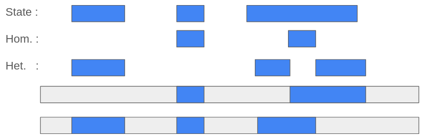
Figure 3: Naming of the called segments in the type column.
chrom  start   end     score        target  type   map         pos        id      map_end     pos_end    id_end  len    map_len     pos_len    nscore
1      7352    8455    99.127010    AFRNEA  het    36.760000   19184015   7352    42.275000   22643831   8455    1103   5.515000    3459816    0.089870
1      47205   47979   72.983646    AFRNEA  het    236.025000  217356752  47205   239.895000  221257830  47979   774    3.870000    3901078    0.094294
1      14808   15393   55.264982    AFRNEA  het    74.040000   48226810   14808   76.965000   54369374   15393   585    2.925000    6142564    0.094470
1      50930   51464   49.448453    AFRNEA  het    254.650000  233984167  50930   257.320000  234906868  51464   534    2.670000    922701     0.092600
1      49458   49854   37.247516    AFRNEA  het    247.290000  230142184  49458   249.270000  231273184  49854   396    1.980000    1131000    0.094059
1      543     956     34.198481    AFRNEA  het    2.715000    3467027    543     4.780000    4089283    956     413    2.065000    622256     0.082805
1      44726   45217   30.486520    AFRNEA  het    223.630000  208767924  44726   226.085000  210563695  45217   491    2.455000    1795771    0.062091
1      54433   54727   26.948920    AFRNEA  het    272.165000  241326256  54433   273.635000  241810161  54727   294    1.470000    483905     0.091663
1      45717   45886   15.501402    AFRNEA  het    228.585000  212806999  45717   229.430000  213596175  45886   169    0.845000    789176     0.091724
1 48255 48389 10.877327 AFRNEA het 241.275000 223011019 48255 241.945000 223649605 48389 134 0.670000 638586 0.081174- ${output}.res.xz : simulated runs of ancestry. Last column indicates the iteration. A summary of this file can be found in another output file, names .res2.xz where ancestry and its overall estimated proportion throughout the genome is given with maximum and minimum estimates. However, the estimates in .res2.xz file also contains the ILS. Overall ancestry proportion can be calculated form the .res.xz file as described in the next section.
state  chrom  start  end    len    it
AFR    1      0      499    499    0
AFR    1      0      539    539    0
AFR    1      500    1364   864    0
AFR    1      1366   1443   77     0
AFR    1      958    1512   554    0
AFR    1      1570   1666   96     0
AFR    1      1667   1937   270    0
AFR    1      1938   2417   479    0
AFR    1      2419   2601   182    0
AFR    1      1487   2905   1418   0
11.2.0.5 Filtering and checking the output files
It is important to make sure the segments detected by admixfrog are real segments. Incomplete lineage sorting (ILS) might be incorrectly detected as an introgressed segment. In most publications only segments with a minimum length of 0.2 cM are retained for very ancient individuals (such as early modern humans) and 0.05 cM for more recent ancient and present day humans.
Overall Neandertal ancestry can be calculated from the ${output}.res.xz file after filtering this file for ILS as following:
res=read.csv("output.res.xz")
res_len_it = res %>% filter(state=='NEA', len>=40)
# len 10 for 0.05 cM and 40 for 0.2 cM

# filtering out the ILS in the called Neandertal segments
res_Nead_sumlen = res_len_it %>% group_by(it) %>% mutate(sum_len_NEA=sum(len))
res_Nead_sumlen = res_Nead_sumlen %>% summarize(it, sum_len_NEA) %>% filter(row_number()==1)

# filtering out the ILS in all called segments
res_all_sumlen = res %>% filter(len>=40) %>% group_by(it) %>% mutate(sum_len_ALL=sum(len))
res_all_sumlen = res_all_sumlen %>% summarize(it, sum_len_ALL) %>% filter(row_number()==1)

# calculating the ratio of Neandertal vs. all segments, per iteration

res_cat = left_join(res_Nead_sumlen, res_all_sumlen) %>%
  mutate(nea_all_ratio = sum_len_NEA/sum_len_ALL, specimen = "Specimen_name")

# maximum and minimum estimates from all iterations:
max(res_cat$nea_all_ratio) # 0.0312594
min(res_cat$nea_all_ratio) # 0.02978274
mean(res_cat$nea_all_ratio) # 0.0303691
11.2.0.6 Limitations of admixfrog
Short segments might not be called or called with high false positive rate.
Run penalty, which determines how often the segments are broken down, needs to be provided by the used. A run penalty that is too conservative (0.1) could break the real segments while a run penalty that is not conservative enough (0.4) could merge separate segments together. The best penalty to use depends on the age of the target genome, and the expected length of the segments. Best practice currently is running admixfrog with different run penalties and comparing the results. Alternative ways of merging/breaking segments is currently being developed.
For the genomes of relatively recent individuals, segment calling results depend a lot on the recombination map used. For older specimens (e.g. early modern humans) the effect of recombination map is small. Best practice currently is running admixfrog with different recombination maps and comparing the results.
Better assignment for deeply divergent references, drop in performance when the references are not deeply diverged. Can result in possible missasignment of ancestries as seen sometimes with Denisovan segments are being called as Neandertal in present day populations.
Better assignment when reference and actual source population are close. For example, the Denisovan populations that introgressed into modern humans are not well represented by the Denisova3 high-coverage genome that is used as the reference representing the Denisovans. This makes the detection of the Denisovan segments challenging.