wfsim <- function(n, g, x0) {
  res <- numeric(g + 1)
  res[1] <- x0
  for (i in 2:(g + 1)) {
    res[i] <- (rbinom(1, n, res[i - 1])) / n
  }
  return(res)
}7 Measuring population structure using Fst
7.1 Theory primer
7.1.1 Genetic drift
Genetic drift is the process by which allele frequencies change randomly due to random fluctuations. Various models exist to model such fluctuations, but the most widely used one is the Wright-Fisher model. In that model, a parent generation of N individuals produces exactly N individuals as offspring, which make up the next generation. To model the fluctuations, every “child” gets assigned a random “parent” from the previous generation.
Example: With \(N=100\) (haploid individuals), we might consider a genetic locus with two alleles \(A\) and \(B\), and in the parent generation, say, 50 individuals carried allele A, and 50 carried allele B. Then, the number of individuals carrying B in the next generation is the number of children who get assigned a parent with allele B. These will be close to 50, but not exactly, due to noise.
As a statistical process, this amounts to a binomial process, where the N offspring individuals are drawn with replacement, each carrying a 50% probability to have A vs. B. In the third generation, this probability may then have already shifted away from 50.
Here is a simple function in R to model the allele frequency in a number of \(g\) successive generations, given a (haploid) population size \(n\) and a starting frequency \(x0\):
We can test it:
set.seed(1)
wfsim(100, 10, 0.5)
[1] 0.50 0.52 0.56 0.46 0.45 0.47 0.48 0.61 0.60 0.58 0.61So indeed the allele frequency changes randomly. We can visualise it for more generations:
time_series <- wfsim(100, 100, 0.5)
plot(time_series, type = "l", ylim = c(0, 1),
     xlab = "generation", ylab = "allele frequency")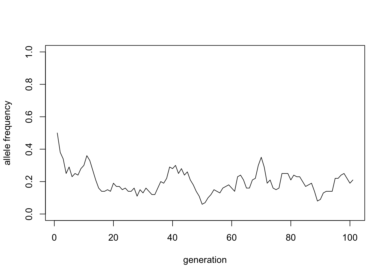
We can better understand this random process, by simulating it many times and plotting the results together:
gens <- 100
sims100 <- replicate(50, wfsim(100, gens, 0.5))
matplot(sims100, type = "l", lty = 1, col = "black",
        ylim = c(0, 1),
        xlab = "generation", ylab = "allele frequency")
This shows how the variance increases with time, and eventually more and more of these curves get absorbed at either \(x=0\) or \(x=1\), a process called “fixation”.
How does this process depend on the population size? We can take a look. Here are three families of simulations, with three different population sizes:
gens <- 1000
sims100 <- replicate(50, wfsim(100, gens, 0.5))
par(mfrow = c(1, 3))
matplot(sims100, type = "l", lty = 1, col = "black",
        xlim = c(0, 100), ylim = c(0, 1),
        xlab = "generation", ylab = "allele frequency", main = "N = 100")

sims1000 <- replicate(50, wfsim(1000, gens, 0.5))
matplot(sims1000, type = "l", lty = 1, col = "black",
        xlim = c(0, 100), ylim = c(0, 1),
        xlab = "generation", ylab = "allele frequency", main = "N = 1000")

sims10000 <- replicate(50, wfsim(10000, gens, 0.5))
matplot(sims10000, type = "l", lty = 1, col = "black",
        xlim = c(0, 100), ylim = c(0, 1),
        xlab = "generation", ylab = "allele frequency", main = "N = 10000")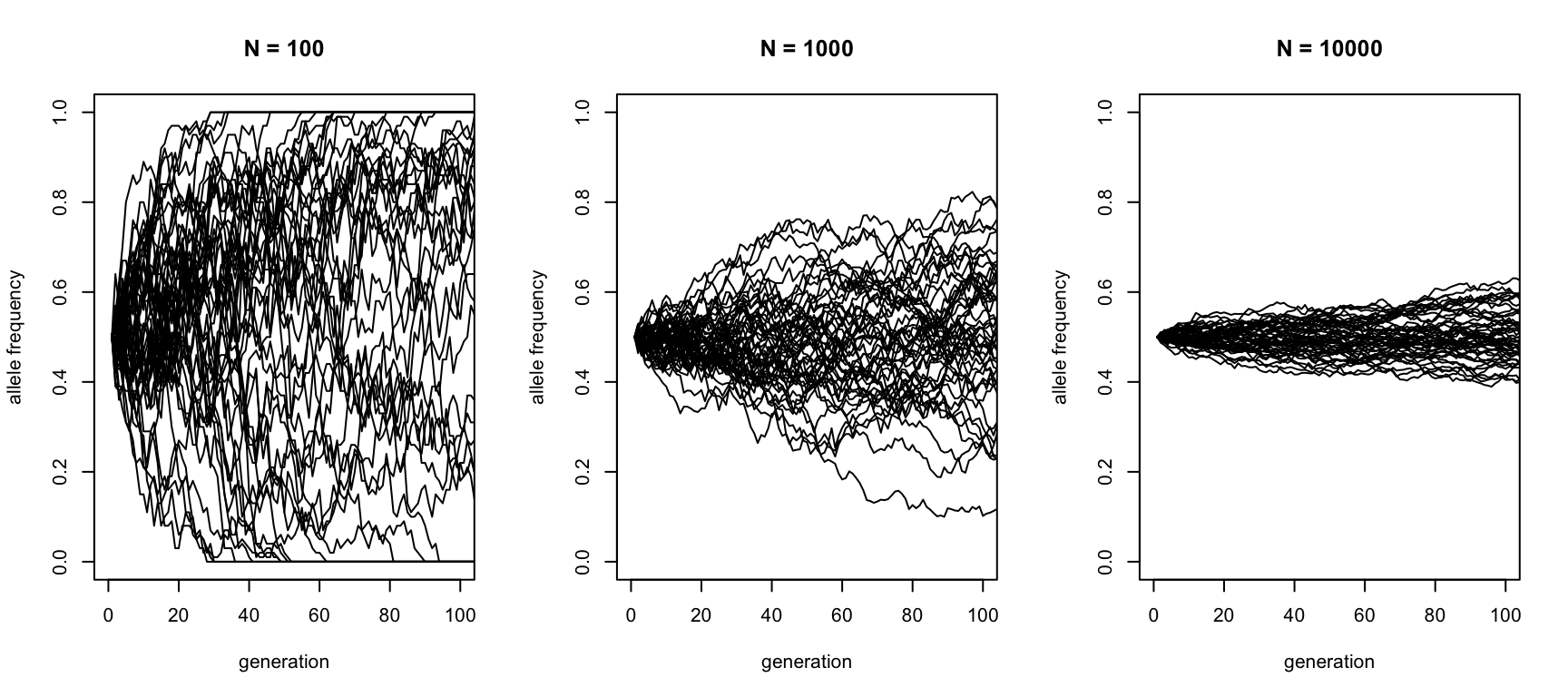
This shows that larger populations have weaker fluctuations than small populations.
7.1.2 \(F_\text{ST}\) quantifies genetic drift
To quantify genetic drift, we can measure the variance of this process over time. The following plot uses the same data as shown above and estimates the variance:
par(mfrow = c(1, 3))
plot(apply(sims100,   1, var), type = "l", ylim = c(0, 0.25),
     xlab = "generations", ylab = "Variance", main = "N = 100")
plot(apply(sims1000,  1, var), type = "l", ylim = c(0, 0.25),
     xlab = "generations", ylab = "Variance", main = "N = 1000")
plot(apply(sims10000, 1, var), type = "l", ylim = c(0, 0.25),
     xlab = "generations", ylab = "Variance", main = "N = 10000")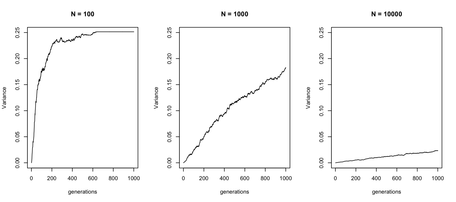
so an increasing variance. But it doesn’t go up forever, but reaches a plateau. This is because of fixation: Once all curves reach fixaton at either \(x=0\) or \(x=1\), variance does no longer increase. In fact, the maximum variance corresponds to the state where all curves have been fixed. The variance to that state corresponds to the variance of a Bernoulli-process, which is \(x_0(1-x_0)\), so it depends on the starting frequency.
It is this plateau of the variance that defines \(F_\text{ST}=1\)! Here is an illustration using again three families of simulations, but this time with the same population size but different starting frequencies:
sims_x05 <- replicate(1000, wfsim(100, gens, 0.5))
sims_x03 <- replicate(1000, wfsim(100, gens, 0.3))
sims_x02 <- replicate(1000, wfsim(100, gens, 0.2))

plot_dat <- cbind(
  apply(sims_x05, 1, var),
  apply(sims_x03, 1, var),
  apply(sims_x02, 1, var)
)

par(mfrow = c(1, 1))

cols <- c("blue", "red", "green")
matplot(plot_dat, type = "l", ylim = c(0, 0.25), lty = 1,
             xlab = "generations", ylab = "Variance", col = cols)
legend(x = "bottomright",
       legend = c("x = 0.5", "x = 0.3", "x = 0.2", "FST = 1"),
       lty = c(1, 1, 1, 2), col = c(cols, "black"))

theory_values <- sapply(c(0.5, 0.3, 0.2), function(x) x * (1 - x))
abline(h = theory_values, lty = 2, col = cols)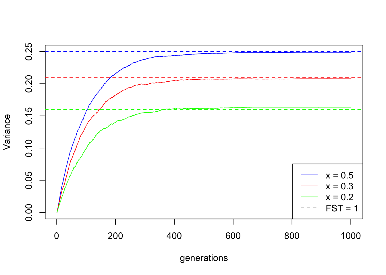
7.1.3 Formal definition of \(F_\text{ST}\)
(Weir and Hill 2002) (explained and summarised in (Bhatia et al. 2013)) give a more formal evolutionary definition of \(F_\text{ST}\), in terms of covariance between derived and ancestral populations. Specifically, for a given SNP, the definition involves the conditional probability of allele frequency \(p_i\) in population \(i\), given an ancestral allele frequency \(p_\text{anc}\), which is defined as a random process with the expectation
Weir, B S, and W G Hill. 2002. “Estimating f-Statistics.” Annual Review of Genetics 36: 721–50. https://doi.org/10.1146/annurev.genet.36.050802.093940.
\[E(p_i|p_\text{anc}) = p_\text{anc}\]
and variance \[Var(p_i|p_\text{anc}) = F_\text{ST}^i p_\text{anc}(1-p_\text{anc}).\]
This form of the conditional variance can be understood by analysing the equation for the two boundary cases: For \(F_\text{ST}^i=0\), there is no variance, so the conditional probability of the derived frequency will be completely determined by the ancestral frequency with no random change. In contrast \(F_\text{ST}^i=1\) means that the variance in the derived allele frequency is that of a binomial distribution with variance \(p_\text{anc}(1-p_\text{anc})\), indicating random but complete fixation of the frequency to 0 or 1.
\(F_\text{ST}\) between two populations A and B is then defined as \[F_\text{ST}(A,B) = \frac{F_\text{ST}^A+F_\text{ST}^B}{2}\].
7.1.4 Estimating \(F_\text{ST}\) from genomic data
All of the above considerations were made using only a single population. But when we usually measure \(F_\text{ST}\), we measure it between two populations. While there are various mathematical definitions for both the theoretical definition and estimation for \(F_\text{ST}\), which differ in subtle ways, we here follow the excellent paper by (Bhatia et al. 2013), which proposes the following estimator, termed Hudson-estimator, which in turn is based on a proposal by (Hudson, Slatkin, and Maddison 1992) and has been implemented in the ADMIXTOOLS package (Patterson et al. 2012):
Hudson, R R, M Slatkin, and W P Maddison. 1992. “Estimation of Levels of Gene Flow from DNA Sequence Data.” Genetics 132 (2): 583–89. https://doi.org/10.1093/genetics/132.2.583.
\[F_\text{ST}=1-\frac{H_w}{H_b}\]
Here, \(H_w\) is the average heterozygosity within each population, and \(H_b\) is the average heterozygosity between two populations. We can easily read off the two boundaries of the definition: At the lower end, we have \(F_\text{ST}=0\) if and only if \(H_w=H_b\), so there is no difference between heterozygosity measured within or between groups, which is equivalent to saying that the two populations are the same. On the upper end we have \(F_\text{ST}=1\) if and only if \(H_w=0\), so all observed variants are fully fixed in both populations (but not necessarily different between the populations).
It is fairly straight forward to see (and shown in (Bhatia et al. 2013)) that the Hudson-estimator above can be recast as
Bhatia, G, N Patterson, S Sankararaman, and A L Price. 2013. “Estimating and Interpreting FST: The Impact of Rare Variants.” Genome Research 23 (9): 1514–21. http://genome.cshlp.org/cgi/doi/10.1101/gr.154831.113.
\[F_\text{ST}(A,B)=\frac{(a-b)^2}{a(1-b)+b(1-a)}\]
Here, \(a\) and \(b\) denote population allele frequencies, which are in principle unobserved, but can be approximated by sample allele frequencies. This approximation is biased, and (Patterson et al. 2012) gives additional formulae for an (asympotically) unbiased estimator (which is for example also used in Poseidon’s tool xerxes, as detailed in the whitepaper).
From this definition, you can see that \(F_\text{ST}(A,B)\) is closely related to F2-statistics, introduced in (Patterson et al. 2012):
\[F_2(A,B)=(a-b)^2\].
In some sense, \(F_\text{ST}(A,B)\) can be considered a normalised version of \(F_2(A,B)\). While both statistics range mathematically from 0 to 1, the upper bound 1 has very different meanings in both. A theoretical value of \(F_2=1\) would mean that both populations are fixed at different alleles in all studied SNPs, which is practically not possible (even completely random fixations would suggest that 1/4 of them would agree given that there are only four nucleotides, let alone the fact that such deeply diverged populations/species would not be alignable anymore). One can say that the time-scale on which \(F_2\) approaches 1, for non-ascertained SNPs, so the entire genome, is the time scale of nucleotide substitutions (i.e. mutations plus fixation) along species branches, which in neutral evolution is given by the inverse mutation rate \(1/\mu\). This would mean something on the order of \(10^8\) generations, which is arguably of the same order of magnitude as the depth of the entire tree of life. In contrast, \(F_\text{ST}\) approaches 1 on the time-scale of fixation of standing variation, which is \(2N\) generations, which for humans is on the order of 10000 generations, so around the depth of modern-human diversity from its origins in Africa several hundred thousand years ago. Arguably, this time scale is much more useful for data analyses and thus easier to interpret.
Of course, in practice, one uses some ascertained SNP set, as also here in our examples below, in which case values are much higher because we consider only variants that are segregating in human populations within a relatively high allele frequency.
If you’ve gone through our chapter on F3 and F4 statistics, you will have already encountered our software xerxes. You can compute both the biased and the approximately unbiased estimators for \(F_\text{ST}(A,B)\), using the FST or FSTvanilla statistics, as defined in the whitepaper.
For what follows, we will use the approximately unbiased form FST.
\(F_\text{ST}(A,B)\) has a convenient and untuitive scale: It ranges from 0 to 1, where \(F_\text{ST}(A,B)=0\) denotes that \(A\) and \(B\) are the same population, with no differentiation whatsoever. On the other hand of the spectrum we have \(F_\text{ST}(A,B)=1\), which would mean that two populations are fully separated.
Another way to see this measure is to consider it as relative shared variance: If you consider genetic variation between \(A\) and \(B\), and within each of \(A\) and \(B\), then \(F_\text{ST}(A,B)\) can be considered to measure the average variance between populations relative to the average variance within populations, again with intuitive boundaries 0 and 1.
7.2 Computing FST using xerxes
For human present-day populations, we can compute pairwise FSt using xerxes.
We here chose a number of populations from (Patterson et al. 2012) with more than 10 samples per population, and prepare the following config file for xerxes:
Patterson, Nick, Priya Moorjani, Yontao Luo, Swapan Mallick, Nadin Rohland, Yiping Zhan, Teri Genschoreck, Teresa Webster, and David Reich. 2012. “Ancient Admixture in Human History.” Genetics 192 (3): 1065–93. https://doi.org/10.1534/genetics.112.145037.
fstats:
- type: FST
  a: ["Adygei", "Balochi", "Basque", "BedouinA", "BedouinB", "Biaka", "Brahui", "Burusho", "Druze", "French", "Han", "Hazara", "Italian_North", "Japanese", "Kalash", "Karitiana", "Makrani", "Mandenka", "Mayan", "Mozabite", "Orcadian", "Palestinian", "Papuan", "Pathan", "Pima", "Russian", "Sardinian", "Sindhi_Pakistan", "Yakut", "Yoruba"]
  b: ["Adygei", "Balochi", "Basque", "BedouinA", "BedouinB", "Biaka", "Brahui", "Burusho", "Druze", "French", "Han", "Hazara", "Italian_North", "Japanese", "Kalash", "Karitiana", "Makrani", "Mandenka", "Mayan", "Mozabite", "Orcadian", "Palestinian", "Papuan", "Pathan", "Pima", "Russian", "Sardinian", "Sindhi_Pakistan", "Yakut", "Yoruba"]
- type: F2
  a: ["Adygei", "Balochi", "Basque", "BedouinA", "BedouinB", "Biaka", "Brahui", "Burusho", "Druze", "French", "Han", "Hazara", "Italian_North", "Japanese", "Kalash", "Karitiana", "Makrani", "Mandenka", "Mayan", "Mozabite", "Orcadian", "Palestinian", "Papuan", "Pathan", "Pima", "Russian", "Sardinian", "Sindhi_Pakistan", "Yakut", "Yoruba"]
  b: ["Adygei", "Balochi", "Basque", "BedouinA", "BedouinB", "Biaka", "Brahui", "Burusho", "Druze", "French", "Han", "Hazara", "Italian_North", "Japanese", "Kalash", "Karitiana", "Makrani", "Mandenka", "Mayan", "Mozabite", "Orcadian", "Palestinian", "Papuan", "Pathan", "Pima", "Russian", "Sardinian", "Sindhi_Pakistan", "Yakut", "Yoruba"]
This will then produce all combinations of \(FST(A, B)\) and \(F_2(A, B)\) as indicated in the population lists.
Note
Note that the config-file engine in xerxes always computes all the combinations of populations, even for cases of \(A=B\). It also doesn’t know about symmetry, so will happily compute the redundant statistics \(FST(\text{Adygei}, \text{Adygei})\) and \(FST(\text{Adygei}, \text{Adygei})\). While this could be possibly improved, there is no big harm done, as this runs fairly quickly.
We run this config file using the command line
REPO=/path/to/community-archive/2012_PattersonGenetics

xerxes fstats -d $REPO --statConfig fstat_world_config.yaml -f fstat_world_output.tsv > fstat_world_table.txt
Note
Please see the Poseidon chapter on how to download Poseidon data from the community archive, as referenced in the following example
The standard output, is a nicely layouted ASCII Table, which looks like this in the beginning:
.-----------.-----------------.-----------------.---.---.---------.----------------.--------------------.------------------.--------------------.
| Statistic |        a        |        b        | c | d | NrSites | Estimate_Total | Estimate_Jackknife | StdErr_Jackknife | Z_score_Jackknife  |
:===========:=================:=================:===:===:=========:================:====================:==================:====================:
| FST       | Adygei          | Adygei          |   |   | 593124  | 0.0000         | 0.0000             | 0.0000           | NaN                |
| FST       | Adygei          | Balochi         |   |   | 593124  | 1.2789e-2      | 1.2789e-2          | 3.3572e-4        | 38.09517110646904  |
| FST       | Adygei          | Basque          |   |   | 593124  | 1.8790e-2      | 1.8790e-2          | 4.0141e-4        | 46.810358341103225 |
| FST       | Adygei          | BedouinA        |   |   | 593124  | 1.3017e-2      | 1.3017e-2          | 2.9647e-4        | 43.90737238689979  |
| FST       | Adygei          | BedouinB        |   |   | 593124  | 3.3455e-2      | 3.3454e-2          | 5.7648e-4        | 58.03217592610529  |
| FST       | Adygei          | Biaka           |   |   | 593124  | 0.1716         | 0.1716             | 1.2185e-3        | 140.85275693678508 |
| FST       | Adygei          | Brahui          |   |   | 593124  | 1.4644e-2      | 1.4644e-2          | 3.4481e-4        | 42.46989237781921  |
| FST       | Adygei          | Burusho         |   |   | 593124  | 1.8566e-2      | 1.8566e-2          | 3.8156e-4        | 48.6573908240317   |
| FST       | Adygei          | Druze           |   |   | 593124  | 1.2173e-2      | 1.2173e-2          | 2.6659e-4        | 45.65975464203526  |
| FST       | Adygei          | French          |   |   | 593124  | 9.7730e-3      | 9.7730e-3          | 3.1627e-4        | 30.9006924987833   |
| FST       | Adygei          | Han             |   |   | 593124  | 9.8759e-2      | 9.8759e-2          | 1.1973e-3        | 82.48660429503893  |
| FST       | Adygei          | Hazara          |   |   | 593124  | 3.0725e-2      | 3.0726e-2          | 7.1478e-4        | 42.98629834431124  |
| FST       | Adygei          | Italian_North   |   |   | 593124  | 8.6600e-3      | 8.6601e-3          | 2.7883e-4        | 31.058813893781032 |
but of course has many more lines (>1800 in this case). We also used the -f flag to output a tab-separated file, here named fstat_world_output.tsv, which is easier to read into R.
7.3 Plotting results in R
All of the following code uses strictly only base-R for maximum compatibility. The code should run on any R installation.
We first load the data
dat <- dat <- subset(read.table("fst_working/fstat_world_output.tsv", sep="\t", header = TRUE),
                     select=-c(c, d, Z_score_Jackknife))
datFST <- dat[dat$Statistic == "FST",]
datF2 <- dat[dat$Statistic == "F2",]
head(datFST)
Statistic a b NrSites Estimate_Total Estimate_Jackknife
1 FST Adygei Adygei 593124 0.000000 0.000000
2 FST Adygei Balochi 593124 0.012789 0.012789
3 FST Adygei Basque 593124 0.018790 0.018790
4 FST Adygei BedouinA 593124 0.013017 0.013017
5 FST Adygei BedouinB 593124 0.033455 0.033454
6 FST Adygei Biaka 593124 0.171600 0.171600
StdErr_Jackknife
1 0.00000000
2 0.00033572
3 0.00040141
4 0.00029647
5 0.00057648
6 0.00121850Ok, this looks good. Let’s check out the largest values
head(dat[order(-dat$Estimate_Total),]) Statistic a b NrSites Estimate_Total Estimate_Jackknife
166 FST Biaka Karitiana 593124 0.3021 0.3021
456 FST Karitiana Biaka 593124 0.3021 0.3021
473 FST Karitiana Papuan 593124 0.3011 0.3011
676 FST Papuan Karitiana 593124 0.3011 0.3011
468 FST Karitiana Mandenka 593124 0.2798 0.2798
526 FST Mandenka Karitiana 593124 0.2798 0.2798
StdErr_Jackknife
166 0.0016933
456 0.0016933
473 0.0026493
676 0.0026493
468 0.0017116
526 0.0017116which shows that the largest FST values of around 0.3 are observed between Karitiana, from South America, and Biaka from Papua Neu Guinea (but note that these values are dependent on the ascertainment of SNPs, which here causes inflation)
Here is a histogram of the values
hist(datFST$Estimate_Total, xlab = "FST", ylab = "Nr of pairs",
     main = "")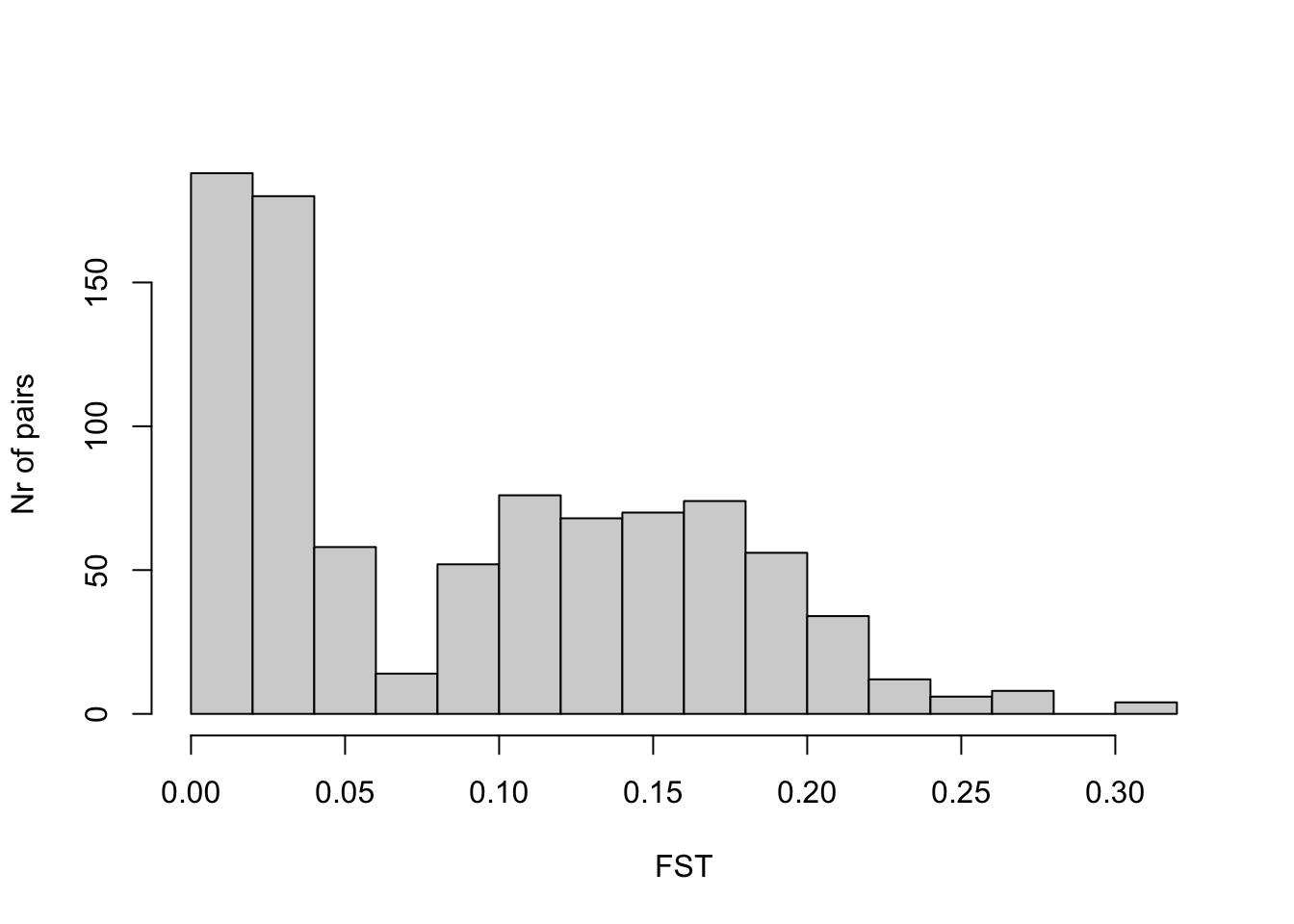
So most values are in the range of a few percent and 20 percent, with a mean of
mean(datFST$Estimate_Total)[1] 0.09015616We can compare that to F2:
hist(datF2$Estimate_Total, xlab = "F2", ylab = "Nr of pairs",
     main = "")
which is an order of magnitude smaller.
So one of the key things to visualise is the pairwise matrix of FST, which we can quickly compute using the xtabs function from the stats package (part of base R):
fstMat <- xtabs(Estimate_Total ~ a + b, datFST)
f2Mat <- xtabs(Estimate_Total ~ a + b, datF2)
and plot a simple heatmap using the powerful heatmap function from the stats package:
heatmap(fstMat, symm = TRUE, hclustfun = function(m) hclust(m, method="ward.D2"))
which we can compare to the output using F2, which looks almost the same:
heatmap(f2Mat, symm = TRUE, hclustfun = function(m) hclust(m, method="ward.D2"))
OK, let’s look at the dendrogram a bit closer:
fstDist <- as.dist(fstMat)
dendro <- hclust(fstDist, method="ward.D2")
plot(dendro, hang = -1, ylab = "FST", xlab = "", main = "")
which again shows the strong drift that Native American populations (Karitiana) and Mayans experienced in their ancestral past.
This nicely shows how FST is affected by total drift, which is inversely proportional to population size, and proportional to total divergence time. A long branch can be caused by either low population size (as in the ancestral population of indigenous Americans) or long divergence time (as between populations from Africa and those outside of Africa).